Clarification of terms
Segmentation means dividing an image into segments or regions based on certain characteristics, such as colour, intensity, texture or edges. Its purpose is to divide images into reasonable parts to make them easier to analyse. In classification, pixels or regions of a photograph are grouped into predefined classes based on certain characteristics. Clustering is the process of grouping data by their appearance, without a predefined list of categories. It is a machine learning technique that aims to find natural groups in the data.
CCA
Binary images can be easily segmented in two steps. In the first step, the algorithm looks at the neighbours of each white pixel from top to bottom, from left to right. If they are all background, a new label is assigned to the current pixel. If a neighbour is not background and is identical, then the current pixel's label gets the label from that neighbour. If there are foreground neighbours with different labels, the lowest label is assigned and then the equivalence is remembered. The second step relabels matching pixels based on the equivalences.
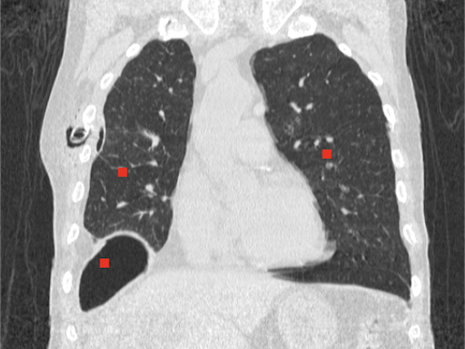
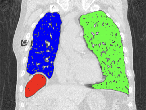
Region growing
The algorithm grows regions starting from selected points based on the similarity of neighbouring pixels. It is important to properly specify a tolerance, which is the allowed percentage difference between pixels. A list of neighbours to be visited is created, then their neighbours are also added to the list, pixels already visited are removed from the list. The process continues until the list is completely empty.
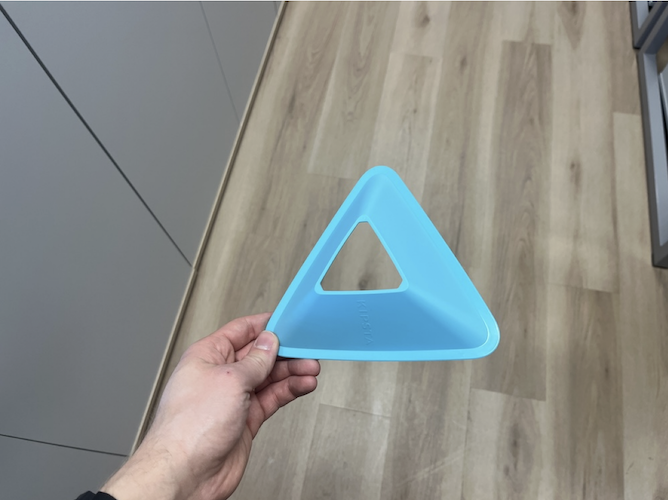
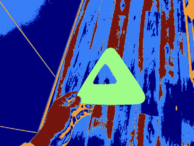
K-means
An iterative clustering method that can be used for image segmentation. The algorithm randomly selects K centroids, then assigns each pixel to the closest cluster based on pixel intensity or other features. Then, the algorithm calculates new centroids based on the average position of the pixels in each cluster. This process is repeated until cluster centers no longer change significantly. Pixels with similar properties are grouped into clusters so that different regions can be separated.
Other algorithms
There are several other methods for segmenting images. Watershed treats the data as a topographic map, interpreting lighter areas as highlands and darker areas as valleys. It can be useful for segmenting complex, touching objects. Certain unsupervised machine learning methods like DBSCAN or Mean-Shift do not require a predefined number of clusters and are well suited for a variety of data structures. Image segmentation with Convolutional Neural Networks is popular in self-driving vehicles, healthcare and many other fields.
Help
Install scikit-learn: https://pypi.org/project/scikit-learn
Ovals image: Download
Chest tube image: Download
Cone image: Download
Source code: CCA
from PIL import Image
import numpy as np
import matplotlib.pyplot as plt
from skimage.measure import label
from skimage.color import label2rgb

# Open the image using PIL
image = Image.open("path-to-resources/ovals.jpeg").convert("L")

# Convert image to a NumPy array
data = np.array(image, dtype=np.uint8)

# Apply thresholding
threshold = 128
data = np.where(data > threshold, 0, 1)

# Label connected regions (CCA)
labels_from_image = label(data)
# Produce an image where labels are color-coded
image_label_overlay = label2rgb(labels_from_image, image=data, alpha=1.0)

# Display the image
plt.imshow(image_label_overlay)
plt.title("Center point")
plt.axis('off')
plt.show()
Source code: Region growing
from PIL import Image
import numpy as np
import matplotlib.pyplot as plt

# Open the image using PIL
# Image source: Case courtesy of Tariq Walizai, Radiopaedia.org, rID: 184833
# https://radiopaedia.org/cases/184833?lang=us
image = Image.open("path-to-resources/chest-tube.jpg").convert("RGB")

# Convert image to a NumPy array
data = np.array(image, dtype=np.uint8)
# Create a grayscale version, as well
grayscale_data = np.array(image.convert("L"), dtype=np.uint8)

seed_points = [[135,235],
                [360,215],
                [115,335]] # (X,Y) coordinates of points

color_values = [(255, 0, 0),
                (0, 255, 0),
                (0, 0, 255)] # (R, G, B)

# Create empty matrix to track visited points
visited_points = np.zeros((data.shape[1], data.shape[0]), dtype=np.uint8)

segmented_image = data.copy()

# Max. difference between pixels (%)
tolerance = 2

for p in range(len(seed_points)):
    temp_list = [seed_points[p]]
    while (len(temp_list) != 0):
        curr_point = temp_list.pop() # Read then remove the last element of the list
        x = curr_point[0]
        y = curr_point[1]
        im_val = grayscale_data[y][x] # Pixel value at the current point
        visited_points[y][x] = 1 # Mark current point white
        segmented_image[y][x] = color_values[p]
        # Visit every neighbor (8c)
        neighbors = [(x-1, y-1), (x-1, y+1), (x+1, y-1), (x+1, y+1), (x, y-1), (x, y+1), (x-1, y), (x+1, y)]
        for i, j in neighbors:
            if (0 <= j < data.shape[0] and 0 <= i < data.shape[1]): # The X and Y index are inside the image
                neighbor_val = grayscale_data[j][i]
                # Change the data type for proper subtraction
                neighbor_val = neighbor_val.astype(np.int16)
                # The point has not been visited and is similar to its neighbor
                if (visited_points[j][i] == 0 and abs(neighbor_val - im_val) < tolerance / 100 * 255 ):
                    # LIFO method
                    temp_list.append([i,j])

# Display the image
plt.imshow(segmented_image)
# Mark seed points
plt.plot(seed_points[0][0], seed_points[0][1], "ow", markersize=5)
plt.plot(seed_points[1][0], seed_points[1][1], "ow", markersize=5)
plt.plot(seed_points[2][0], seed_points[2][1], "ow", markersize=5)
plt.title("Center point")
plt.axis('off')
plt.show()
Source code: K-means
from PIL import Image
import numpy as np
import matplotlib.pyplot as plt
from sklearn.cluster import KMeans

# Open the image using PIL
image = Image.open("path-to-resources/cone.jpg")

# Convert image to a NumPy array
data = np.array(image, dtype=np.uint8)

# Get the dimensions of the image
image_h, image_w, _ = data.shape

# Reshape image data for k-means
pixels = data.reshape(-1, 3)
# Run the k-means algorithm
kmeans = KMeans(n_clusters = 4)
kmeans.fit(pixels)

# Get labels
labels = np.reshape(kmeans.labels_, (image_h, image_w))

# Display images
fig, ax = plt.subplots(1, 2, figsize=(12, 6))
ax[0].imshow(data)
ax[0].set_title("Original Image")
ax[0].axis("off")
ax[1].imshow(labels, cmap = "jet")
ax[1].set_title("Segmented Image")
ax[1].axis("off")
plt.show()