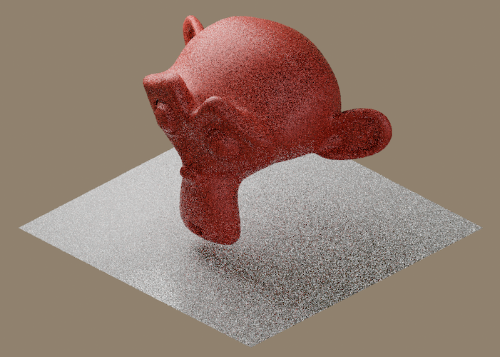
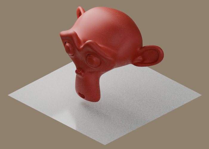
Denoising
One of the unwanted changes in photographs is noise, which is difficult to filter out afterwards because it is hard not to blur the details. Methods have to find and remove noise, which are differences between adjacent pixels, while retaining important edges, which are also differences between adjacent pixels. Machine learning is widely used today to filter noise. These algorithms have learned what is noisy and what is clean on millions of images, but a number of classical methods are also used.
Median filter
For each pixel with a given neighbourhood the algorithm finds the median, the middle value of the ordered list of values. This will be the new value of the pixel. Since it tries to retain the most characteristic colour at each location, it does not wash out edges but does remove noise. It is very sensitive to the window size.
Bilateral filter
It is essentially a Gaussian blur, but the effect of the convolution kernel's elements is weighted based on the intensity difference measured relative to the current pixel. Homogeneous parts are subject to the smoothing effect, while significant edges are left untouched. Its speed is highly dependent on the window size and was named after its two-step (bilateral) nature.
Total variation
The total variation itself is the sum of the changes, the gradients of the image. This noise filtering method aims to create an image with a lower TV, while still looking very similar to the original image. Several good algorithms exist to solve this problem, one of the most popular being the Chambolle-Pock algorithm.
Wavelet
The wavelet transform is similar to the Fourier transform, but it also preserves local information, meaning it not only calculates what frequencies are present in the image, but also their location. After the transform, the data is broken down into components, followed by a threshold operation, and then finally an inverse wavelet transform results in an image where edges are preserved and unwanted noise is removed.
Non-local means
It tries to remove noise by analysing the whole image, rather than just neighbours of the actual pixel. It not only weights based on nearby similar regions, but also on similar regions in any part of the image. NLM is computationally expensive, but often gives a nicer, more usable result than other methods.
Ray-tracing noise
Ray-tracing has become a well-known concept thanks to the marketing of GPU manufacturers (Nvidia, AMD), but it has been used for decades by designers, editors, film studios. In Ray-tracing (RT for short), a ray starts from the camera and when it collides with an object, the algorithm calculates the light interactions, like the reflection, refraction, shadow, global illumination. The final result can be approximated by averaging millions of rays. One drawback of ray-tracing is that the statistical fluctuations due to random patterns lead to noisy results. For example Pixar and SolidWorks use Nvidia's Optix RT engine and AI denoiser in their softwares.
Help
Install PyWavelets: https://pypi.org/project/PyWavelets
Spore image: Download
Source code: Denoising methods
from PIL import Image
import numpy as np
import matplotlib.pyplot as plt
from skimage.filters import median
from skimage.restoration import denoise_bilateral, denoise_tv_chambolle, denoise_wavelet, denoise_nl_means

# Open the image using PIL
image = Image.open("path-to-resources/noisy-items.png").convert("L")

# Convert image to a NumPy array
data = np.array(image, dtype = np.uint8)

# Footprint for the median filter
custom_footprint = np.array([[1, 1, 1, 1, 1],
                              [1, 1, 1, 1, 1],
                              [1, 1, 1, 1, 1],
                              [1, 1, 1, 1, 1],
                              [1, 1, 1, 1, 1]], dtype = np.uint8)

# Perform denoising using various algorithms
denoised_image_med = median(data, footprint = custom_footprint)
denoised_image_bl = denoise_bilateral(data, sigma_color = 0.05, sigma_spatial = 5)
denoised_image_tv = denoise_tv_chambolle(data, weight = 0.1)
denoised_image_wl = denoise_wavelet(data)
denoised_image_nlm = denoise_nl_means(data, h = 0.1, fast_mode = "True", patch_size = 5, patch_distance = 6)

# Display images
filters = [
    ("Original Image", data),
    ("Median filter", denoised_image_med),
    ("Bilateral filter", denoised_image_bl),
    ("Total variation", denoised_image_tv),
    ("Wavelet", denoised_image_wl),
    ("Non-local means", denoised_image_nlm)
]
fig, axes = plt.subplots(2, 3, figsize=(12, 8))
for ax, (title, img) in zip(axes.ravel(), filters):
    ax.imshow(img, cmap="gray")
    ax.set_title(title)
    ax.axis("off")
plt.tight_layout()
plt.show()